uark_enrollment <- data.frame(
  year = c(2012, 2013, 2014, 2015, 2016, 2017, 2018, 2019, 2020, 2021, 2022, 2023, 2024),
  full_time = c(19508, 20379, 21047, 21415, 21668, 22144, 22602, 22193, 22070, 23282, 25214, 28426, 29886),
  part_time = c(5029, 4962, 5190, 5339, 5526, 5414, 5176, 5366, 5492, 5786, 5722, 3714, 3724)
)
uark_enrollment$total <-
  uark_enrollment$full_time + uark_enrollment$part_time

# Make sure the data is sorted by year
uark_enrollment <- sort_by(uark_enrollment, uark_enrollment$year)7 Time to work with Times
In preparation for the remainder of the course, we will be thinking about working with data that is arranged in time. To do so, we are going to practice working with dates in R.
7.1 Years
The simplest time-series data to deal with is annual data. For example, take uark_enrollment below.
In this setting, year is just another regular numeric variable. Let’s create a plot of enrollment over time. To do so, plot year on the x-axis and total on the y-axis.
plot(total ~ year, data = uark_enrollment)
If I want to connect these points, I can add the type = "l" argument to plot. Or, if I want both lines and points, I can use type = "b" (for “both”).
plot(total ~ year, data = uark_enrollment, type = "l")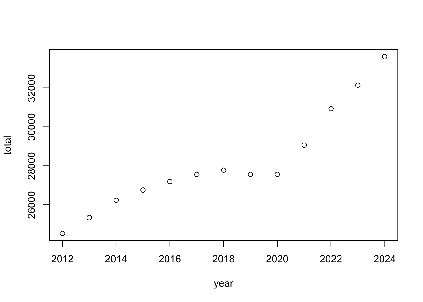
plot(total ~ year, data = uark_enrollment, type = "b")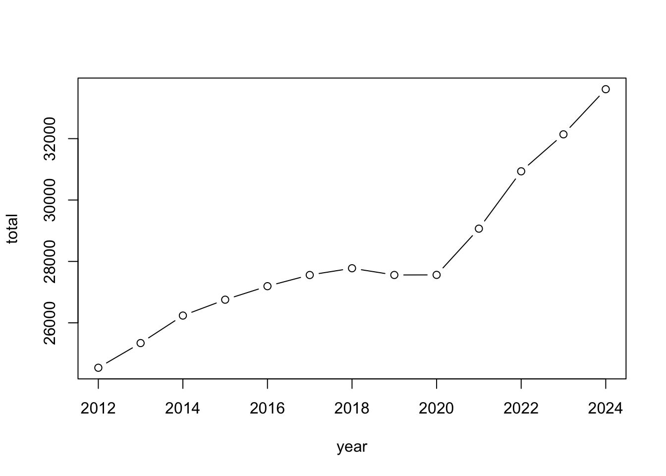
7.2 Working with dates
However, when we get to dates (day month year), this gets more difficult. Here we have box scores from Arkansas football’s 2023 season, but note the days are written as strings
# Arkansas' 2023 football games
football <- data.frame(
  date = c(
    "11-11-2023", "11-04-2023", "09-23-2023", "09-02-2023", "10-07-2023",
    "09-16-2023", "09-09-2023", "10-21-2023", "11-24-2023", "10-14-2023",
    "11-18-2023", "09-30-2023"
  ),
  month = c(11, 11, 9, 9, 10, 9, 9, 10, 11, 10, 11, 9),
  day = c(11, 4, 23, 2, 7, 16, 9, 21, 24, 14, 18, 30),
  year = rep(2023, 12L),
  school = rep("Arkansas", 12L),
  opponent = c(
    "Auburn", "Florida", "(12) LSU", "Western Carolina", "(16) Ole Miss", "BYU",
    "Kent State", "Mississippi State", "(10) Missouri", "(11) Alabama",
    "Florida International", "Texas A&M"
  ),
  result = c("L", "W", "L", "W", "L", "L", "W", "L", "L", "L", "W", "L"),
  pts = c(10, 39, 31, 56, 20, 31, 28, 3, 14, 21, 44, 22),
  pts_opponent = c(48, 36, 34, 13, 27, 38, 6, 7, 48, 24, 20, 34)
)
For example, say I wanted to plot the points scored by Arkansas over the season. Trying to use date will create a problem since it’s a character
plot(pts ~ date, data = football)Error in plot.window(...): need finite 'xlim' valuesI can try with month or day, but both are wrong. For example, if I use day on the x-axis, these are not in the correct order.
plot(pts ~ month, data = football)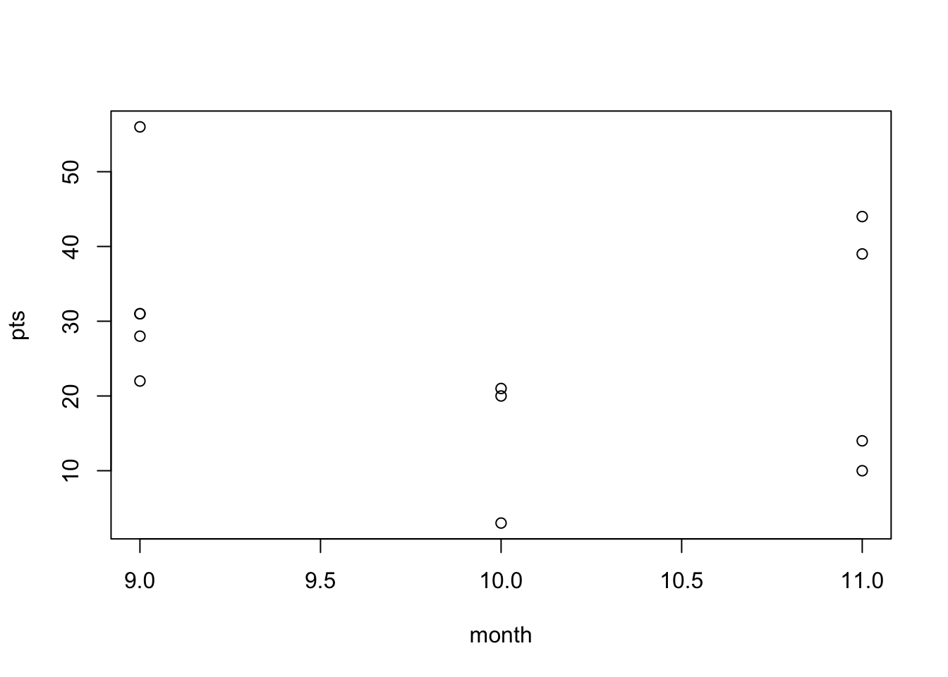
plot(pts ~ day, data = football)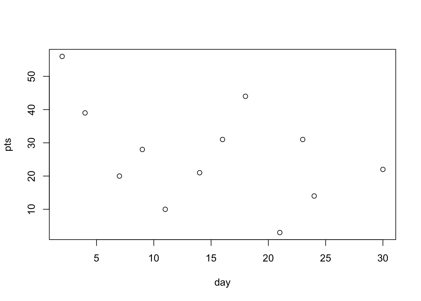
The best I could think to do is to kind of fake it by doing
## approximately converts to days since January 1st
plot(football$month * 30 + football$day, football$pts)
7.3 Dates in R
It turns out R has a bunch of functionality to work with dates built in. But, I think the easiest way to work with dates is to use the lubridate package, so let’s load that library.
## You might need to install this.
## To do so, run this:
## install.packages("lubridate")
library(lubridate)
Attaching package: 'lubridate'The following objects are masked from 'package:base':
date, intersect, setdiff, unionlubridate has a bunch of functions to help work with dates. First, we have date() which creates a Date object in R
today <- today()
class("2025-08-22")
[1] "character"class(today)[1] "Date"Note the order I am writing this: year-month-day. This is called the ISO Date format. ISO is the “International Organization for Standardization” and is a group that sets standards for all kinds of measurements. I LOVE this format. One reason is that if you have strings containing the dates and sort those strings, they will sort chronologically as well! Month/day/year does not have this feature (it would group same days on different years).
Internally, R represents dates as a number! But a very strange number:
as.numeric(today)[1] 20389Because dates are represented a number, we need a day “0”. If we used the first day BC as the 0, then most modern days would be really big numbers. When computers were much smaller, this could create problems, so they went with January 1st, 1970 as day 0 (or “1970-01-01”).
today - date("1970-01-01")Time difference of 20389 daysYou can add and subtract days from Date objects. 1 is a single day.
tomorrow <- today + 1
two_days_ago <- today - 2
cat(paste0("Today is ", today, ". Tomorrow is ", tomorrow, "."))
Today is 2025-10-28. Tomorrow is 2025-10-29.Dates and the date function work as vectors too:
last_4_classes <- date(c("2025-10-22", "2025-10-20", "2025-10-15", "2025-10-13"))
print(last_4_classes)
[1] "2025-10-22" "2025-10-20" "2025-10-15" "2025-10-13"7.3.1 Back to football dataset
So returning to our previous problem, we can convert our string of dates to actual dates. But, if we try with date, we will get an error:
date(football$date)This is because the date is in an ambiguous format. It does not know if “11-04-2023” is November 4th or April 11th.
Instead, lurbidate has a set of functions mdy, myd, dmy, dym, ymd, ydm that allow you to tell R what order the year, month, and day are in. There are 6 possible combinations and 6 functions.
## Convert to date
football$date <- mdy(football$date)
football$date
[1] "2023-11-11" "2023-11-04" "2023-09-23" "2023-09-02" "2023-10-07"
[6] "2023-09-16" "2023-09-09" "2023-10-21" "2023-11-24" "2023-10-14"
[11] "2023-11-18" "2023-09-30"Now we can plot our scores over time. and look, R will print out pretty labels!!
plot(pts ~ date, data = football)
But, you might notice something weird if you use type = "l" or type = "b"
plot(pts ~ date, data = football, type = "b")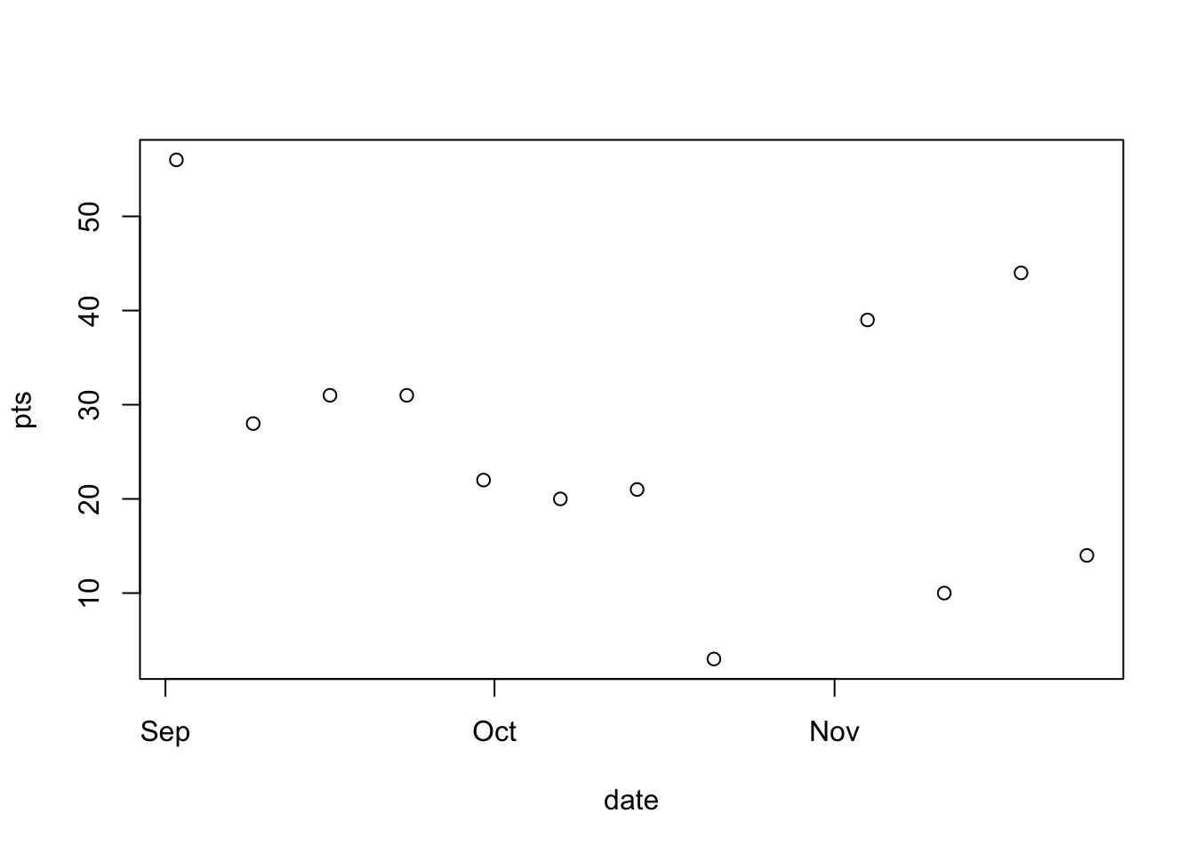
The problem occurs because our data is not sorted. When a line is being plotted, it will connect points in the order they appear in the data set. It is very important to sort you data when working with time-series data!
football <- sort_by(football, ~date)

## equivalent to
## football <- sort_by(football, football$date)
## football <- sort_by(football, football$year, football$month, football$day)
## football <- football[order(football$date), ]plot(pts ~ date, data = football, type = "b")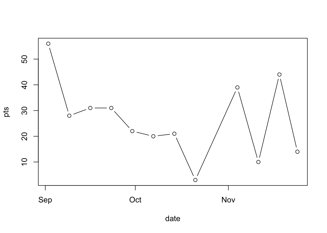
7.3.2 More lubridate functions
Okay, say we have a vector of Dates. I can use lubridate’s year()/month()/day() functions to extract the components.
Try the month function out on football$date. What happens if you add the argument label = TRUE option to month?
year(football$date) [1] 2023 2023 2023 2023 2023 2023 2023 2023 2023 2023 2023 2023month(football$date) [1] 9 9 9 9 9 10 10 10 11 11 11 11month(football$date, label = TRUE) [1] Sep Sep Sep Sep Sep Oct Oct Oct Nov Nov Nov Nov
12 Levels: Jan < Feb < Mar < Apr < May < Jun < Jul < Aug < Sep < ... < Dec## day of month =
day(football$date) [1] 2 9 16 23 30 7 14 21 4 11 18 24mday(football$date) [1] 2 9 16 23 30 7 14 21 4 11 18 24## day of year = days since january 1
yday(football$date) [1] 245 252 259 266 273 280 287 294 308 315 322 328## day of the week
wday(football$date) [1] 7 7 7 7 7 7 7 7 7 7 7 6wday(football$date, label = TRUE) [1] Sat Sat Sat Sat Sat Sat Sat Sat Sat Sat Sat Fri
Levels: Sun < Mon < Tue < Wed < Thu < Fri < Satwday(football$date, week_start = "Monday") [1] 6 6 6 6 6 6 6 6 6 6 6 5## Quarters Q1, Q2, Q3, Q4
quarter(football$date) [1] 3 3 3 3 3 4 4 4 4 4 4 4## Year + Quarter
quarter(football$date, type = "year.quarter") [1] 2023.3 2023.3 2023.3 2023.3 2023.3 2023.4 2023.4 2023.4 2023.4 2023.4
[11] 2023.4 2023.47.3.2.1 Exercise
What is the most common month in the football dataset? Hint: use the table function to help.
7.4 Unemployment data
Let’s introduce a new dataset on the rate of unemployment in the US.
unemployment <- read.csv("data/unemployment.csv")

# Convert `date` string into a `Date`:
unemployment$date <- ymd(unemployment$date)
unemployment <- sort_by(unemployment, ~date)
Now, let’s make a time-series plot of the unemployment rate over time
plot(unrate ~ date, data = unemployment, type = "l")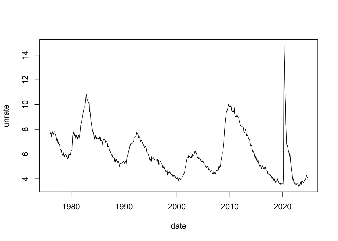
7.4.1 Calculating autocorrelation of unemployment rate
To calculate the autocorrelation between \(y_{t}\) and \(y_{t-1}\), we need to “shift” y back by one. Of course, the first period does not have a lag! So we will append an NA at the start like this: c(NA, ...).
Do this to create the variable unemployment$unrate_lag1
## Number of time-periods
T <- nrow(unemployment)

## Get y_{t-1}
unemployment$unrate_lag1 <-
  c(NA, unemployment$unrate[1:(T - 1)])

## Get y_{t-2}
unemployment$unrate_lag2 <-
  c(NA, NA, unemployment$unrate[1:(T - 2)])

## Get y_{t-3}
unemployment$unrate_lag3 <-
  c(NA, NA, NA, unemployment$unrate[1:(T - 3)])

## Grab last-years values, y_{t-12}
unemployment$unrate_lag12 <-
  c(
    rep(NA, 12),
    unemployment$unrate[1:(T - 12)]
  )
Then, calculate the autocovariance or autocorrelation between unrate and unrate_lag1 using cov or cor
cor(
  x = unemployment$unrate,
  y = unemployment$unrate_lag2,
)
[1] NASimilar to before, if there are NAs present, then NA is returned. Instead of na.rm = TRUE, we need to use the argument use = "complete.obs".
cor(
  x = unemployment$unrate,
  y = unemployment$unrate_lag1,
  use = "complete.obs"
)
[1] 0.9616146## Alternatively, we could grab the correct rows
cor(
x = unemployment$unrate[1:(T - 1)],
y = unemployment$unrate[2:T]
)[1] 0.9616146cor(
x = unemployment$unrate,
y = unemployment$unrate_lag12,
use = "complete.obs"
)[1] 0.65913037.4.2 Quarters
One important variable we might want is the quarter that a date falls within (Q1, Q2, Q3, and Q4). Let’s try to make this using the quarter function from lubridate.
## make new variable in unemployment called `quarter`
unemployment$quarter <- quarter(unemployment$date)

## Keep yourself from accidentally using quarter as a numeric
unemployment$quarter <-
  paste("Q", unemployment$quarter)
7.5 Basic time-series regression
As a preview of what is to come, let’s see which quarter of the year has the lowest unemployment rate:
library(fixest)

## Do not do this
unemployment$q1 <- (quarter(unemployment$date) == 1)
unemployment$q2 <- (quarter(unemployment$date) == 2)
unemployment$q3 <- (quarter(unemployment$date) == 3)
unemployment$q4 <- (quarter(unemployment$date) == 4)
est_bad_version <- feols(
  unrate ~ 0 + q1 + q2 + q3 + q4,
  data = unemployment, vcov = "hc1"
)
The variable 'q4TRUE' has been removed because of collinearity (see
$collin.var).## Use `i`, it prints more nicely and is more simple!
est <- feols(
unrate ~ 0 + i(quarter(date)),
data = unemployment, vcov = "hc1"
)
etable(est) est
Dependent Var.: unrate
quarter(date) = 1 6.063*** (0.1375)
quarter(date) = 2 6.230*** (0.1614)
quarter(date) = 3 6.114*** (0.1409)
quarter(date) = 4 6.072*** (0.1411)
_________________ _________________
S.E. type Heteroskeda.-rob.
Observations 585
R2 -0.00027
Adj. R2 -0.00544
---
Signif. codes: 0 '***' 0.001 '**' 0.01 '*' 0.05 '.' 0.1 ' ' 1Just like with cross-sectional regression, a regression of an outcome on a set of indicator variables (without an intercept) produces a set of averages. If we were to add an intercept, then we would estimate difference in means between groups:
est_w_intercept <- feols(
  unrate ~ 1 + i(quarter(date)),
  data = unemployment, vcov = "hc1"
)
etable(est, est_w_intercept)
est est_w_intercept
Dependent Var.: unrate unrate
quarter(date) = 1 6.063*** (0.1375)
quarter(date) = 2 6.230*** (0.1614) 0.1673 (0.2120)
quarter(date) = 3 6.114*** (0.1409) 0.0510 (0.1968)
quarter(date) = 4 6.072*** (0.1411) 0.0096 (0.1970)
Constant 6.063*** (0.1375)
_________________ _________________ _________________
S.E. type Heteroskeda.-rob. Heteroskeda.-rob.
Observations 585 585
R2 -0.00027 0.00144
Adj. R2 -0.00544 -0.00372
---
Signif. codes: 0 '***' 0.001 '**' 0.01 '*' 0.05 '.' 0.1 ' ' 1Let’s fit a simple time-trend to the data. We can use predict to get fitted values and then add them to the plot using the lines function.
model_linear_trend <- feols(
  unrate ~ date,
  data = unemployment
)
unemployment$unrate_linear_trend <- predict(model_linear_trend)
plot(unrate ~ date, data = unemployment, type = "l")
lines(unrate_linear_trend ~ date, data = unemployment, col = "blue")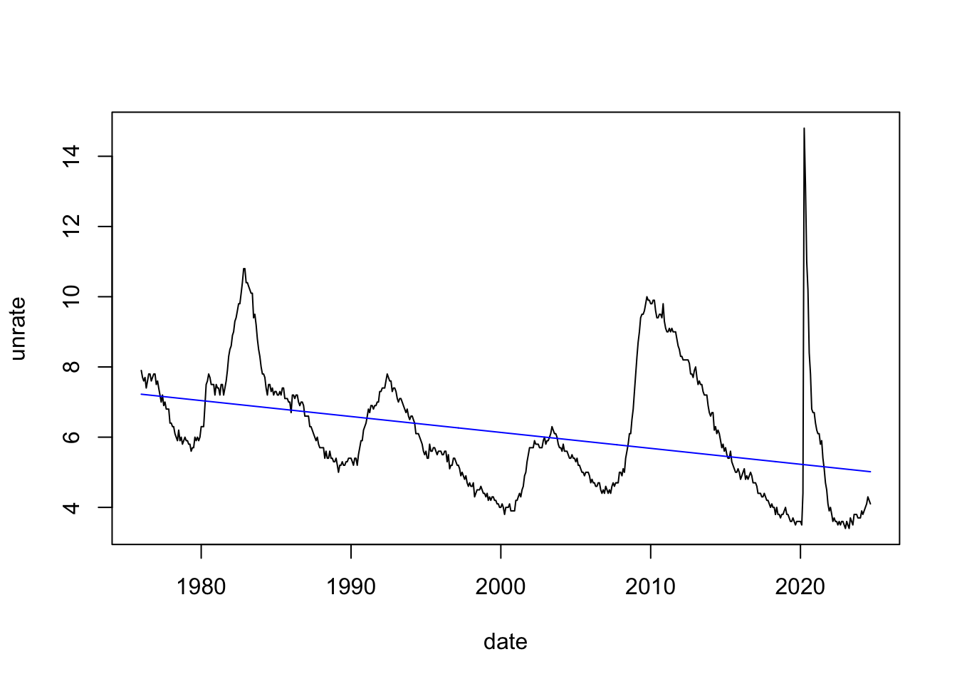
7.6 Exercise
- What were the average numbers of points scored by Arkansas in the 2023 for each month? Use a regression to answer this question