3 Vectors

So far, we have dealth with scalar numbers and texts. But, when working with data, we will observe many units and need a way to store all their values together. This is where the bread and butter of data-science comes in: Vectors.

Vectors are a list of elements like integers, numbers, or strings. This is really useful for storing data! You use c to create a vector (pneumonically, c stands for combine).

## Rebounds from 2023 NBA Season
rebounds <- c(260, 114, 252, 310, 165, 236, 148, 336, 941, 127, 384, 278, 300, 6, 136, 145, 233, 142, 420, 35, 11, 161, 485, 1, 830, 81, 112, 16, 63, 513, 162, 296, 434, 239, 22, 269, 235, 222, 485, 245, 578, 162, 281, 344, 39, 99, 82, 79, 476, 3, 69, 84, 201, 52, 223, 244, 34, 728, 5, 423, 286, 346, 324, 549, 580, 152, 401, 58, 95, 187, 618, 189, 69, 184, 34, 101, 36, 7, 472, 78, 41, 631, 259, 12, 760, 33, 410, 672, 70, 227, 272, 247, 289, 63, 96, 500, 497, 739, 188, 178, 491, 1, 298, 202, 211, 307, 227, 439, 253, 24, 740, 168, 921, 61, 210, 213, 209, 150, 145, 220, 26, 144, 286, 190, 56, 182, 580, 105, 402, 660, 260, 118, 0, 231, 11, 184, 69, 432, 807, 257, 762, 24, 42, 342, 95, 185, 77, 310, 170, 447, 98, 271, 8, 41, 99, 85, 102, 593, 275, 24, 10, 206, 407, 51, 184, 0, 98, 10, 305, 43, 112, 30, 80, 312, 292, 292, 899, 182, 317, 511, 665, 78, 633, 314, 32, 11, 49, 205, 402, 296, 46, 26, 261, 429, 451, 66, 546, 206, 35, 5, 63, 161, 227, 394, 308, 118, 92, 249, 691, 257, 85, 220, 483, 233, 909, 744, 564, 208, 573, 25, 243, 16, 2, 30, 132, 34, 468, 460, 330, 268, 1, 252, 318, 453, 473, 33, 82, 494, 26, 450, 54, 110, 145, 870, 670, 111, 1, 179, 448, 700, 74, 845, 30, 27, 639, 15, 97, 705, 96, 54, 295, 312, 556, 39, 551, 426, 45, 258, 8, 233, 564, 630, 536, 5, 255, 95, 173, 11, 51, 106, 71, 393, 317, 149, 394, 301, 319, 19, 147, 257, 336, 350, 19, 416, 829, 2, 219, 1530, 171, 124, 54, 47, 296, 30, 26, 96, 168, 14, 118, 770, 310, 66, 934, 42, 415, 204, 634, 202, 301, 391, 177, 81, 256, 116, 188, 76, 417, 1, 28, 435, 191, 449, 270, 265, 5, 1, 0, 47, 183, 0, 22, 247, 0, 381, 19, 2, 862, 253, 469, 55, 37, 90, 246, 78, 88, 512, 0, 101, 265, 28, 238, 223, 257, 372, 21, 236, 94, 81, 295, 206, 704, 454, 607, 145, 129, 282, 405, 247, 1258, 15, 269, 9, 240, 260, 305, 75)

It is kind of a pain in the neck to write all these out; and worse, prone to errors! Later, we will learn how to load data from a file, making this much easier.

You can access elements of a vector by using [#], where # is the \(i\)-th element you want

rebounds[1]

[1] 260

rebounds[2]

[1] 114

If you want to access more than one element, we can subset using a vector! (how meta):

rebounds[c(1, 2)]

[1] 260 114

One special syntax is ther a:b which generates \(a, a+1, \dots, b\). This makes it easy to grab the first 5 values:

rebounds[1:5]

[1] 260 114 252 310 165

Standard math operators work on vectors element by element:

rebounds[1:5] + 1

[1] 261 115 253 311 166

rebounds[1:5] / 12 # dozens of rebounds

[1] 21.66667  9.50000 21.00000 25.83333 13.75000

If we want to know how many elements are in a vector, we can use the length function:

length(rebounds)

[1] 386

3.1 Summarizing vectors

The natural next step is to start trying to summarize the data. There are a set of built-in functions that provide statistical summaries of the data.

## Mean, standard deviation, and variance
mean(rebounds)

[1] 250.4663

sd(rebounds)

[1] 232.6362

var(rebounds)

[1] 54119.62

## Extremes
max(rebounds)

[1] 1530

min(rebounds)

[1] 0

## chaining functions
sqrt(var(rebounds))

[1] 232.6362

Some functions will take extra arguments that give more instructions. For example, the quantile function returns information about percentiles of the distribution. You can add extra arguments, separated by commas. For example, quantile’s first argument is a vector and the second argument is what percentiles you want to find.

## Percentiles of the data
quantile(rebounds, c(0.1, 0.5, 0.9))

  10%   50%   90% 
 19.0 205.5 575.5

We will talk in more details about plotting below, but for now we can use the hist() function to give us a view of the distribution of the vector

hist(rebounds)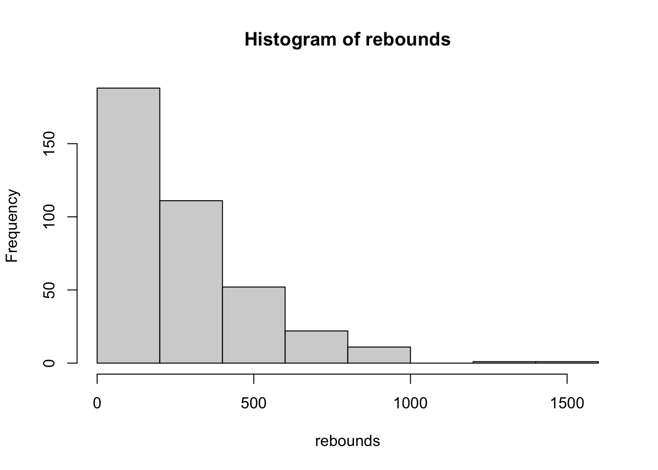

3.1.1 Help menu

How did I know the order of arguments for quantile? Are there ways to customize the histogram created by hist? In general, if you have a question about a function, then you need to address that function’s documentation. To do so, click in to your console and type ?func_name where func_name is the name of the function, e.g. quantile. At first, the information may be very overwhelming. The documentation in base R functions are very detailed, but are not great at introducing the functions. You should focus on the Arguments section and perhaps the Examples section, in my opinion. In particular, the order of the arguments is probably helpful in order of importance

3.1.1.1 Exercise

Similar to c, the seq function creates a vector: a sequence of numbers.

Create a sequence of all multiples of four from 4 to 100. Look at `?seq for help. Hint: The arguments you need here are from, to, and by. Store your vector in a varaible
Find the 19th element of this sequence
What is the sum of the 10th and 11th element of this sequence.

3.1.2 `NA`s

In the real world, some times we will not have a value for a variable for an individual (e.g. people don’t fill answer a survey question). In R, this is represented as an NA.

reviews <- c(5, NA, 4, 4, 3, 5,  NA, 4, 5, 2)

What is the average (mean and median) review?

mean(reviews)

[1] NA

median(reviews)

[1] NA

By default, the statistical summary functions will all produce NA when they are present in the data. R wants you to opt-in to ignoring the missings. To do this, functions will take an extra argument called na.rm:

mean(reviews, na.rm = FALSE)

[1] NA

max(reviews, na.rm = FALSE)

[1] NA

A lot of this information will be presented to you by the summary function. For numberic vectors, summary produces the five-number summary, the mean, and the number of NAs (if any)

summary(reviews)

   Min. 1st Qu.  Median    Mean 3rd Qu.    Max.    NA's 
   2.00    3.75    4.00    4.00    5.00    5.00       2

3.1.3 Logical Vectors

So far, we have seen two kinds of vectors: numeric and character vectors. A third, common, vector is a logical vector:

ordered_takeout <- c(TRUE, TRUE, FALSE, TRUE, FALSE, TRUE, FALSE, FALSE)

Logical vectors can take only two values: TRUE and FALSE. They can be treated as numbers by using as.numeric() with TRUE becoming 1 and FALSE becoming 0.

as.numeric(ordered_takeout)

[1] 1 1 0 1 0 1 0 0

One common trick is to use sum() on a logical vector and it will return the number of TRUEs:

sum(ordered_takeout)

[1] 4

Logical vectors are often returned by other operations. For example, we can check whether elements of a vector equal some value with ==. Other operators that produce a logical vector include >, <, >=, and <=.

## Find five-star reviews
reviews == 5

 [1]  TRUE    NA FALSE FALSE FALSE  TRUE    NA FALSE  TRUE FALSE

## Find three-star or lower 
reviews <= 3

 [1] FALSE    NA FALSE FALSE  TRUE FALSE    NA FALSE FALSE  TRUE

Logical vectors can be negated using the ! operator:

## Find non five-star reviews
!(reviews == 5)

 [1] FALSE    NA  TRUE  TRUE  TRUE FALSE    NA  TRUE FALSE  TRUE

You can also use the following operators to supply multiple criteria:

& And operator. Both vector 1 and vector 2 must be true for the observation
| Or operator. Either vector 1 or vector 2 must be true for the observation

(reviews == 5) & (reviews == 4)

 [1] FALSE    NA FALSE FALSE FALSE FALSE    NA FALSE FALSE FALSE

(reviews == 5) | (reviews == 4)

 [1]  TRUE    NA  TRUE  TRUE FALSE  TRUE    NA  TRUE  TRUE FALSE

## Equivalent to 
reviews >= 4

 [1]  TRUE    NA  TRUE  TRUE FALSE  TRUE    NA  TRUE  TRUE FALSE

3.1.4 Subsetting of vectors by logical

We have already discussed one way of subsetting vectors via a vector of integers. This is called “subsetting by index”.

The other common way is by using a logical vector the same length of the vector you wish to subset. For example, let’s look at the reviews for takeout orders and dine-in orders separately

## Takeout orders
reviews[ordered_takeout]

[1]  5 NA  4  5  5  2

## Dine-in orders
reviews[!ordered_takeout]

[1]  4  3 NA  4

3.1.4.1 Exercise

What is the average review for take-out orders?

The is.na() function takes a vector as an argument and returns a logical vector that equals TRUE if the element is NA. Using this and the !, subset the reviews to only non-NA values. What is the average review? Comapre this to mean(reviews, na.rm = TRUE).

mean(reviews[!is.na(reviews)])

[1] 4

mean(reviews, na.rm = TRUE)

[1] 4

3.1.5 Vectorized operations

Often times we want to use multiple vectors for some calculation. Like single numbers, arithmetic can be done element-by-element with vectors. This means +, -, *, / and ^ all work on a vector.

x <- c(1, 2, 3)
y <- c(5, 5, 5)

x + y

[1] 6 7 8

x^2

[1] 1 4 9

There are two main features to remember: 1. The vectors you use should be of the same length (if they are not, some weird recycling rules occur that we will not discuss in this introduction). 2. Scalars are treated as a vector of the same length with that single number repeated for each element.

## Equivalent:
x + 2

[1] 3 4 5

x + rep(2, 3)

[1] 3 4 5

More, many functions are designed to be used on vectors element by element. All of the functions we used in the “Calculator” section do this:

exp(x)

[1]  2.718282  7.389056 20.085537

log(x)

[1] 0.0000000 0.6931472 1.0986123

sqrt(x^2)

[1] 1 2 3

3.1.5.1 Exercise

Try to guess the output of the following expression 2*x + y + 1.

3.1.6 Sorting data

The final vector operation we will discuss is how to sort data; either ascending or descending in value. There are two ways to do this.

First, we can use the sort() function. The function takes a function and an optional decreasing argument. decreasing takes a logical TRUE/FALSE option. By default, it increases in values

sort(rebounds, decreasing = TRUE)

  [1] 1530 1258  941  934  921  909  899  870  862  845  830  829  807  770  762
 [16]  760  744  740  739  728  705  704  700  691  672  670  665  660  639  634
 [31]  633  631  630  618  607  593  580  580  578  573  564  564  556  551  549
 [46]  546  536  513  512  511  500  497  494  491  485  485  483  476  473  472
 [61]  469  468  460  454  453  451  450  449  448  447  439  435  434  432  429
 [76]  426  423  420  417  416  415  410  407  405  402  402  401  394  394  393
 [91]  391  384  381  372  350  346  344  342  336  336  330  324  319  318  317
[106]  317  314  312  312  310  310  310  308  307  305  305  301  301  300  298
[121]  296  296  296  295  295  292  292  289  286  286  282  281  278  275  272
[136]  271  270  269  269  268  265  265  261  260  260  260  259  258  257  257
[151]  257  257  256  255  253  253  252  252  249  247  247  247  246  245  244
[166]  243  240  239  238  236  236  235  233  233  233  231  227  227  227  223
[181]  223  222  220  220  219  213  211  210  209  208  206  206  206  205  204
[196]  202  202  201  191  190  189  188  188  187  185  184  184  184  183  182
[211]  182  179  178  177  173  171  170  168  168  165  162  162  161  161  152
[226]  150  149  148  147  145  145  145  145  144  142  136  132  129  127  124
[241]  118  118  118  116  114  112  112  111  110  106  105  102  101  101   99
[256]   99   98   98   97   96   96   96   95   95   95   94   92   90   88   85
[271]   85   84   82   82   81   81   81   80   79   78   78   78   77   76   75
[286]   74   71   70   69   69   69   66   66   63   63   63   61   58   56   55
[301]   54   54   54   52   51   51   49   47   47   46   45   43   42   42   41
[316]   41   39   39   37   36   35   35   34   34   34   33   33   32   30   30
[331]   30   30   28   28   27   26   26   26   26   25   24   24   24   22   22
[346]   21   19   19   19   16   16   15   15   14   12   11   11   11   11   10
[361]   10    9    8    8    7    6    5    5    5    5    3    2    2    2    1
[376]    1    1    1    1    1    0    0    0    0    0    0

Alternatively, we can use the order() function to get the row indices of the ordering:

order(rebounds, decreasing = TRUE)

  [1] 298 379   9 313 113 215 177 244 347 252  25 295 139 310 141  85 216 111
 [19]  98  58 258 371 250 209  88 245 181 130 255 317 183  82 272  71 373 158
 [37]  65 127  41 219 217 271 263 265  64 197 273  30 356 180  96  97 238 101
 [55]  23  39 213  49 235  79 349 227 228 372 234 195 240 332 249 150 108 330
 [73]  33 138 194 266  60  19 327 294 315  87 163 377 129 189  67 204 285 282
 [91] 320  11 344 364 292  62  44 144   8 291 229  63 287 233 179 283 184 174
[109] 262   4 148 311 205 106 169 385 286 319  13 103  32 190 303 261 369 175
[127] 176  93  61 123 376  43  12 159  91 152 333  36 381 230 334 359 193   1
[145] 131 384  83 268 140 210 290 363 323 275 109 348   3 232 208  92 342 378
[163] 353  40  56 221 383  34 361   6 366  37  17 214 270 134  90 107 203  55
[181] 362  38 120 212 297 116 105 115 117 218 162 198 370 188 316 104 318  53
[199] 331 124  72  99 325  70 146  74 136 165 339 126 178 248 100 321 277 299
[217] 149 112 307   5  31  42  22 202  66 118 284   7 289  16 119 243 374 122
[235]  18  15 225 375  10 300 132 206 309 324   2  27 171 246 242 280 128 157
[253]  76 358  46 155 151 167 257  95 259 306  69 145 276 367 207 352 355 156
[271] 211  52  47 237  26 322 368 173  48  80 182 354 147 326 386 251 281  89
[289]  51  73 137 196 312  29  94 201 114  68 125 350 241 260 301  54 164 279
[307] 187 302 338 191 267 170 143 314  81 154  45 264 351  77  20 199  57  75
[325] 226  86 236 185 172 224 253 304 329 360 254 121 192 239 305 220 110 142
[343] 160  35 341 365 288 293 345  28 222 256 380 308  84  21 135 186 278 161
[361] 168 382 153 269  78  14  59 200 274 335  50 223 296 346  24 102 231 247
[379] 328 336 133 166 337 340 343 357

The first element of the resulting vector is the index of the maximum number (1530)

order(rebounds, decreasing = TRUE)[1]

[1] 298

which.max(rebounds)

[1] 298

What this means is that we can use the result of order to subset the vector to get the sorted vector:

rebounds[order(rebounds, decreasing = TRUE)]

  [1] 1530 1258  941  934  921  909  899  870  862  845  830  829  807  770  762
 [16]  760  744  740  739  728  705  704  700  691  672  670  665  660  639  634
 [31]  633  631  630  618  607  593  580  580  578  573  564  564  556  551  549
 [46]  546  536  513  512  511  500  497  494  491  485  485  483  476  473  472
 [61]  469  468  460  454  453  451  450  449  448  447  439  435  434  432  429
 [76]  426  423  420  417  416  415  410  407  405  402  402  401  394  394  393
 [91]  391  384  381  372  350  346  344  342  336  336  330  324  319  318  317
[106]  317  314  312  312  310  310  310  308  307  305  305  301  301  300  298
[121]  296  296  296  295  295  292  292  289  286  286  282  281  278  275  272
[136]  271  270  269  269  268  265  265  261  260  260  260  259  258  257  257
[151]  257  257  256  255  253  253  252  252  249  247  247  247  246  245  244
[166]  243  240  239  238  236  236  235  233  233  233  231  227  227  227  223
[181]  223  222  220  220  219  213  211  210  209  208  206  206  206  205  204
[196]  202  202  201  191  190  189  188  188  187  185  184  184  184  183  182
[211]  182  179  178  177  173  171  170  168  168  165  162  162  161  161  152
[226]  150  149  148  147  145  145  145  145  144  142  136  132  129  127  124
[241]  118  118  118  116  114  112  112  111  110  106  105  102  101  101   99
[256]   99   98   98   97   96   96   96   95   95   95   94   92   90   88   85
[271]   85   84   82   82   81   81   81   80   79   78   78   78   77   76   75
[286]   74   71   70   69   69   69   66   66   63   63   63   61   58   56   55
[301]   54   54   54   52   51   51   49   47   47   46   45   43   42   42   41
[316]   41   39   39   37   36   35   35   34   34   34   33   33   32   30   30
[331]   30   30   28   28   27   26   26   26   26   25   24   24   24   22   22
[346]   21   19   19   19   16   16   15   15   14   12   11   11   11   11   10
[361]   10    9    8    8    7    6    5    5    5    5    3    2    2    2    1
[376]    1    1    1    1    1    0    0    0    0    0    0

This might seem like a bit silly, but it will prove useful when we want to sort multiple vectors at the same time based on one of the vectors.