# Count
hist(penguins$body_mass_lb)
Common functions for graphing are hist() for plotting one variable and plot() for plotting two variables.
# Count
hist(penguins$body_mass_lb)
You can add additional commands for better plots. Use ?hist to see the list of options.
?hist into the console and find the following options:Change these to make a more professional histogram:
## Modify this
hist(penguins$body_mass_lb)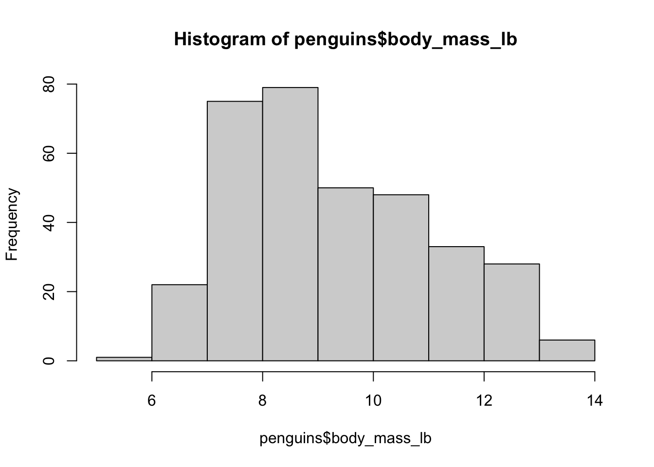
bill_length_mm for Adelie and Chinstrap penguins.While we haven’t talked about this yet, it is typically of interest to compare multiple variables together. To plot two variables, we will use the plot() function to make scatter plots.
plot(penguins$flipper_length_mm, penguins$body_mass_lb, main = "Scatter plot of flipper length and body mass")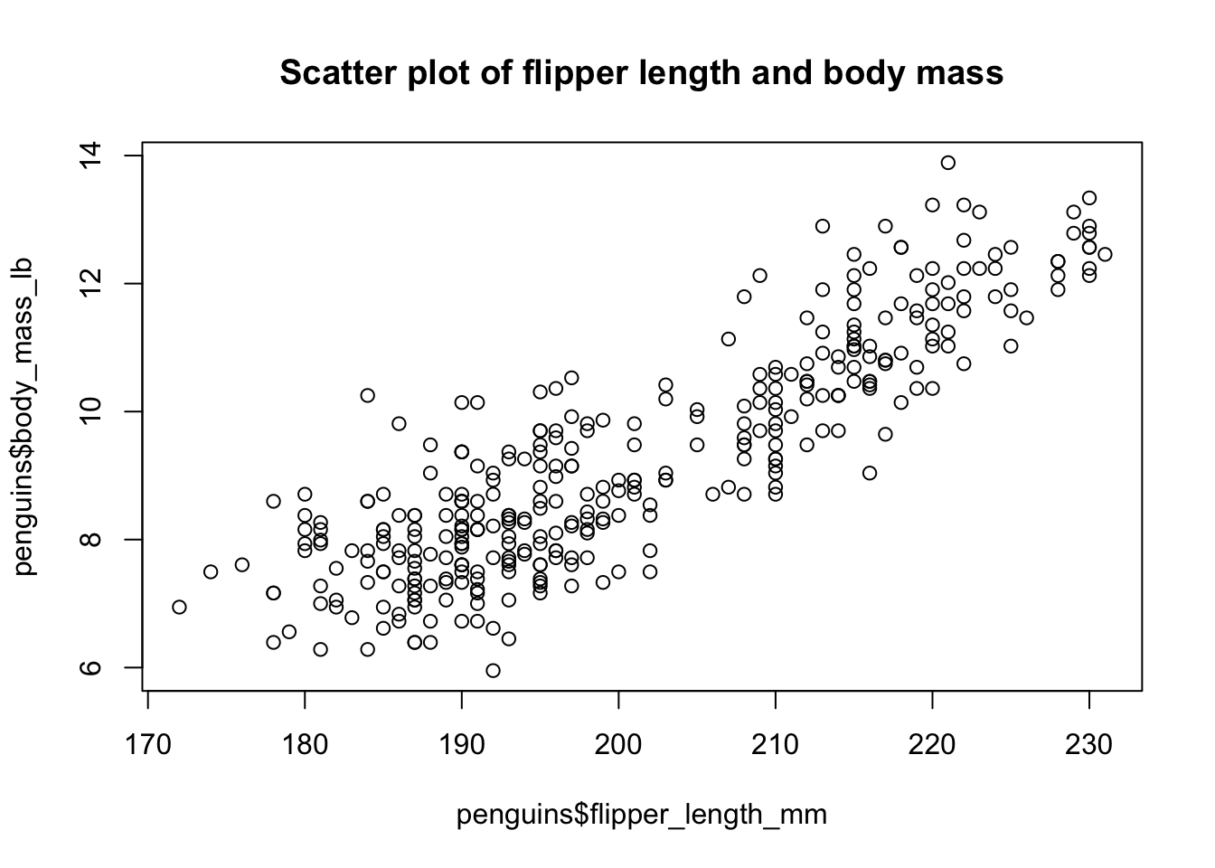
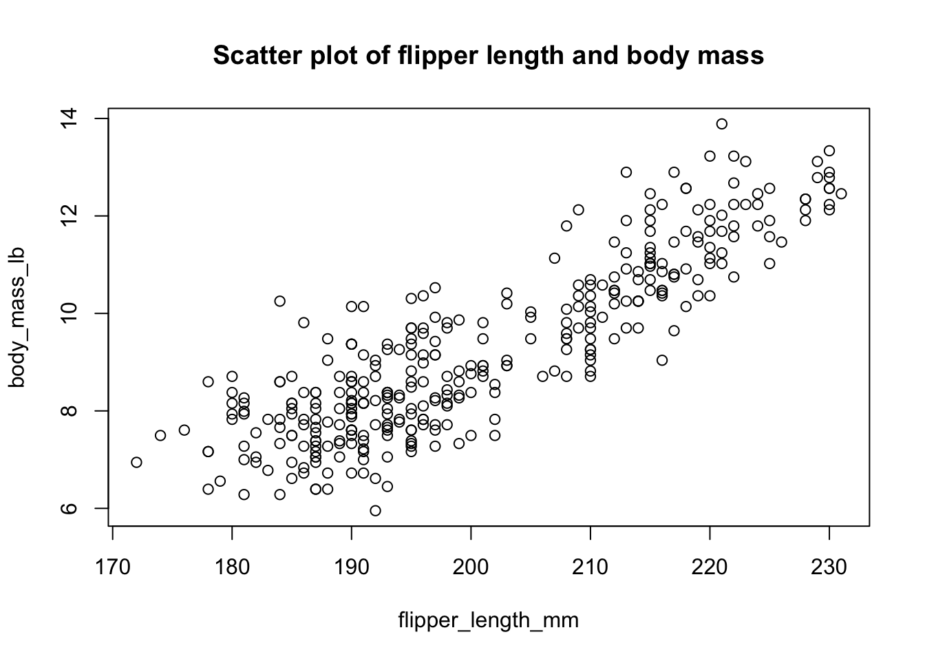
It can be kind of annoying to type penguins$ twice in plot. There is a second way to call plot which uses formula syntax. A formula has the following syntax yvar ~ xvar where yvar and xvar are variable names. So we can use body_mass_lb ~ flipper_length_mm to specify variables and then tell plot to use the penguins data.frame using the data argument.
plot(
  body_mass_lb ~ flipper_length_mm,
  data = penguins,
  main = "Scatter plot of flipper length and body mass"
)
If the data argument is not provided, it will look for body_mass_lb and flipper_length_mm as variables defined in the global environment. If these variables are within a data.frame and not as their own variables, then you will get the “object not found” error again.
The reason I am showing you this is that this syntax will show up again when we run linear regressions in this class. And, in fact, this form of function calling where we use a data argument and then reference variables within that data.frame by name is actually quite common (see dplyr section in advanced materials).
There is a package called ggplot2 that improves base Rs graphing library. We will not cover the details here, but a curious student can find much more details here: https://ggplot2-book.org/
This is a particularly nice introduction: https://uopsych-r-bootcamp-2020.netlify.app/post/06-ggplot2/
library(ggplot2)

## Set custom theme
theme_set(
  theme_minimal() + theme(
  plot.title.position = "plot",
  plot.caption = element_text(hjust = 0, face = "italic"),
  plot.caption.position = "plot",
  legend.position = "top",
  legend.title.position = "top",
  legend.location = "plot",
  legend.margin = margin(0, 0, 5, 0),
  legend.justification = c(0, 1),
  legend.background = element_rect(fill = "white", color = NA),
  legend.key.spacing.x = unit(12, "pt")
))ggplot() +
geom_histogram(
data = penguins,
aes(x = body_mass_lb, color = species, fill = species),
alpha = 0.3
) +
labs(
title = "Histogram of Penguin Body Mass, by species",
x = "Weight (in lb.)",
color = "Species",
fill = "Species"
) +
scale_color_manual(values = c("darkorange", "purple", "cyan4")) +
scale_fill_manual(values = c("darkorange", "purple", "cyan4")) +
theme_minimal()`stat_bin()` using `bins = 30`. Pick better value `binwidth`.Warning: Removed 2 rows containing non-finite outside the scale range
(`stat_bin()`).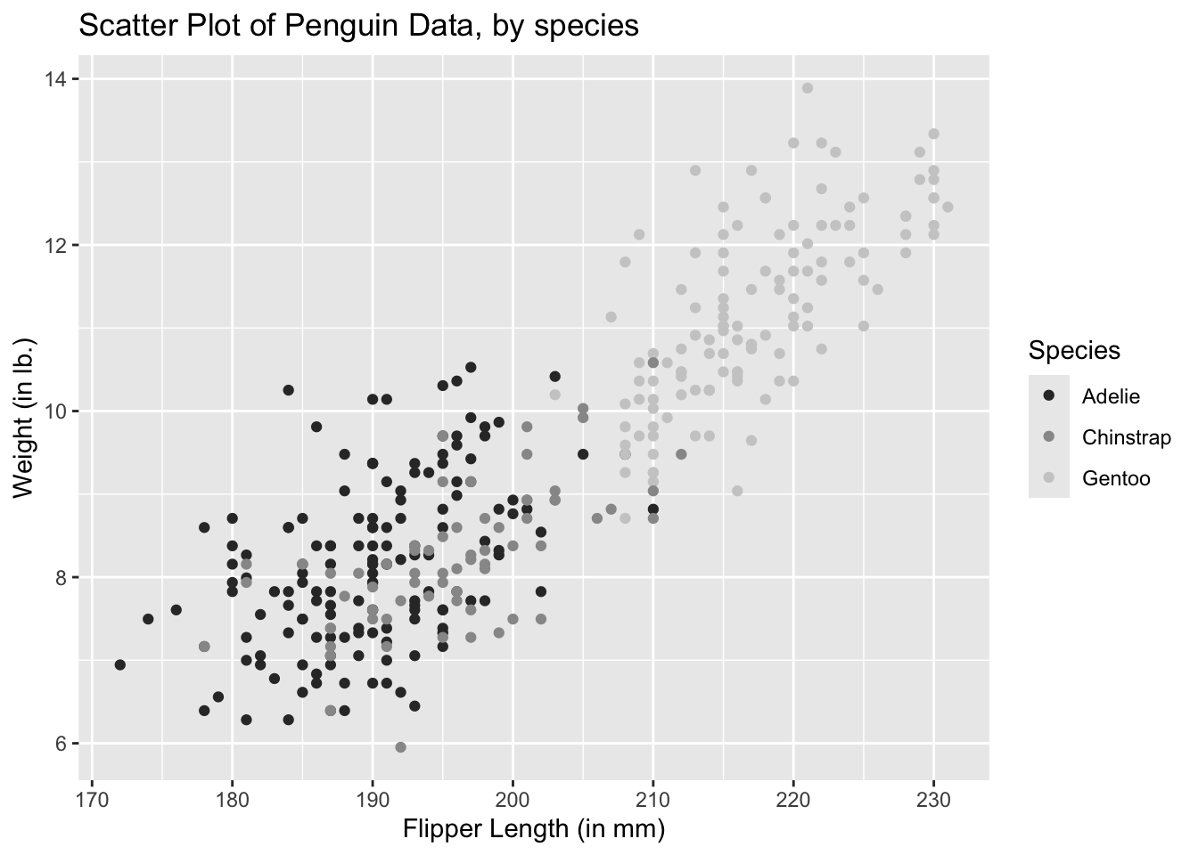
ggplot() +
  geom_point(
    data = penguins,
    aes(x = flipper_length_mm, y = body_mass_lb, color = species)
  ) +
  labs(
    title = "Scatter Plot of Penguin Data, by species",
    x = "Flipper Length (in mm)",
    y = "Weight (in lb.)",
    color = "Species",
    fill = "Species"
  ) +
  scale_color_manual(values = c("darkorange", "purple", "cyan4")) +
  theme_minimal()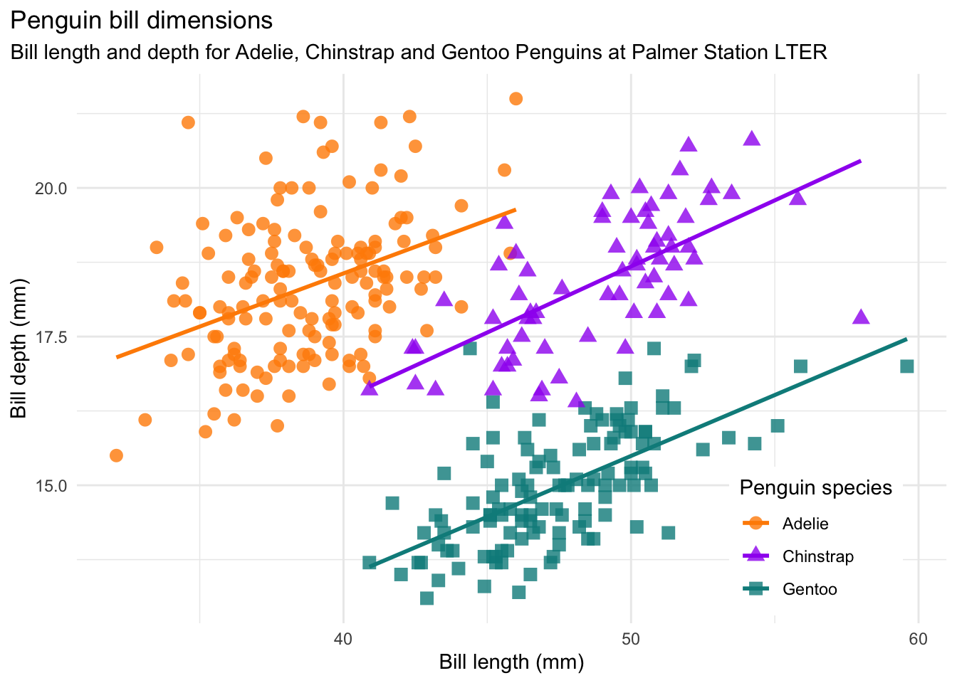
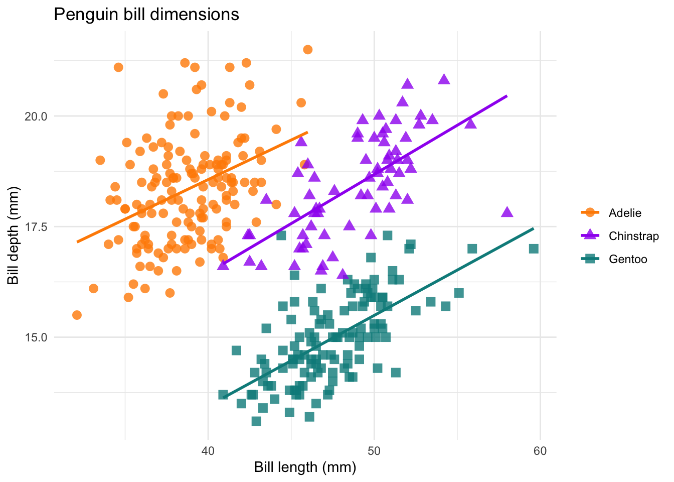
ggplot2 makes it really easy to make beautiful and professional graphs and it would be a really useful skill to have in your career
ggplot(
  data = penguins,
  aes(
    x = bill_length_mm,
    y = bill_depth_mm,
    group = species
  )
) +
  geom_point(
    aes(color = species, shape = species),
    size = 3,
    alpha = 0.8
  ) +
  geom_smooth(method = "lm", se = FALSE, aes(color = species)) +
  theme_minimal() +
  scale_color_manual(values = c("darkorange", "purple", "cyan4")) +
  labs(
    title = "Penguin bill dimensions",
    x = "Bill length (mm)",
    y = "Bill depth (mm)",
    color = NULL,
    shape = NULL
  )
`geom_smooth()` using formula = 'y ~ x'Warning: Removed 2 rows containing non-finite outside the scale range
(`stat_smooth()`).Warning: Removed 2 rows containing missing values or values outside the scale range
(`geom_point()`).