## You might need to install this. To do so, run this:
## install.packages("fixest")
library(fixest)6 Running regressions in R
One of the most common and flexible ways to analyze data is using a linear regression model. While R comes with the lm function to run regressions, I recommend the fixest package. This uses the same syntax as lm but has a bunch of features that make many things simpler and nicer.
To begin, we will use a data set on the SAT scores of NYC public schools
nyc <- read.csv("data/nyc_sat.csv")
str(nyc)
'data.frame': 435 obs. of 22 variables:
$ school_id : chr "02M260" "06M211" "01M539" "02M294" ...
$ school_name : chr "Clinton School Writers and Artists" "Inwood Early College for Health and Information Technologies" "New Explorations into Science, Technology and Math High School" "Essex Street Academy" ...
$ borough : chr "Manhattan" "Manhattan" "Manhattan" "Manhattan" ...
$ building_code : chr "M933" "M052" "M022" "M445" ...
$ street_address : chr "425 West 33rd Street" "650 Academy Street" "111 Columbia Street" "350 Grand Street" ...
$ city : chr "Manhattan" "Manhattan" "Manhattan" "Manhattan" ...
$ state : chr "NY" "NY" "NY" "NY" ...
$ zip_code : int 10001 10002 10002 10002 10002 10002 10002 10002 10002 10002 ...
$ latitude : num 40.8 40.9 40.7 40.7 40.7 ...
$ longitude : num -74 -73.9 -74 -74 -74 ...
$ phone_number : chr "212-695-9114" "718-935-3660 " "212-677-5190" "212-475-4773" ...
$ start_time : chr "" "8:30 AM" "8:15 AM" "8:00 AM" ...
$ end_time : chr "" "3:00 PM" "4:00 PM" "2:45 PM" ...
$ student_enrollment : int NA 87 1735 358 383 416 255 545 329 363 ...
$ percent_white : chr "" "3.4%" "28.6%" "11.7%" ...
$ percent_black : chr "" "21.8%" "13.3%" "38.5%" ...
$ percent_hispanic : chr "" "67.8%" "18.0%" "41.3%" ...
$ percent_asian : chr "" "4.6%" "38.5%" "5.9%" ...
$ average_score_sat_math : int NA NA 657 395 418 613 410 634 389 438 ...
$ average_score_sat_reading: int NA NA 601 411 428 453 406 641 395 413 ...
$ average_score_sat_writing: int NA NA 601 387 415 463 381 639 381 394 ...
$ percent_tested : chr "" "" "91.0%" "78.9%" ...## Looks like NYC :-)
plot(latitude ~ longitude, data = nyc)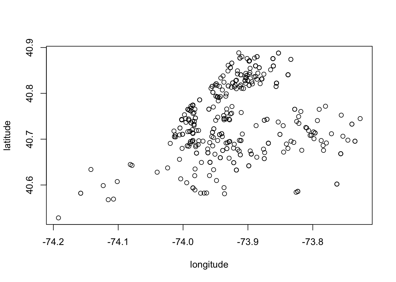
6.0.0.1 Exercise
Whenever working with a new dataset, it is good to plot variables to get a sense of the data. In this class, a lot of data is clean already, but in the wild, you will see a lot of weirdness. For example, the Census Bureau often times codes NA in monthly income as 9999. If you don’t look at the data and instead just run regressions, your results will be really wonky from these “very high income earners”.
To familiarize ourselves with this data, let’s plot a few key variables.
- First, create a histogram of
average_score_sat_mathandaverage_score_sat_reading
- Print out
percent_white; what’s the problem here?
- Create a scatter plot comparing SAT reading score with SAT math score. Please use quality x and y labels. Additionally, use a high-quality title. Try and write a descriptive title that gives your reader a “key takeaway”.
6.1 First regression by hand
First, let’s use some code to fix the percent variables. I simply delete the % from the string and then convert to a number:
nyc$percent_white <- as.numeric(gsub("%", "", nyc$percent_white))
nyc$percent_black <- as.numeric(gsub("%", "", nyc$percent_black))
nyc$percent_hispanic <- as.numeric(gsub("%", "", nyc$percent_hispanic))
nyc$percent_asian <- as.numeric(gsub("%", "", nyc$percent_asian))
nyc$percent_tested <- as.numeric(gsub("%", "", nyc$percent_tested))
Now, let’s do our first regression by hand. We want to regress average SAT reading score on average SAT math score. Recall the formula for the OLS coefficients \(\hat{\beta}_0\) and \(\hat{\beta}_1\) are given by
\[ \hat{\beta}_1 = \text{cov}(X, Y) / \text{var}(X) \ \text { and }\hat{\beta}_0 = \bar{Y} - \bar{X} * \hat{\beta}_1 \]
Let’s grab the math and reading scores and put in variables x and y for ease of writing. But first, we need to drop NAs in either x or y. To do this, we will grab the two columns from nyc and then use the na.omit() function to drop any rows that contain an NA in any variable.
## need to drop NAs manually
vars <- nyc[, c("average_score_sat_math", "average_score_sat_reading")]
vars <- na.omit(vars)
x <- vars$average_score_sat_math
y <- vars$average_score_sat_reading

## No NAs
sum(is.na(x)) + sum(is.na(y))
[1] 0Now, that x and y contain no NAs
## Calcualate regression by hand
ybar <- mean(y)
xbar <- mean(x)
var_x <- var(x)
cov_x_y <- cov(x, y)
beta_1_hat <- cov_x_y / var_x
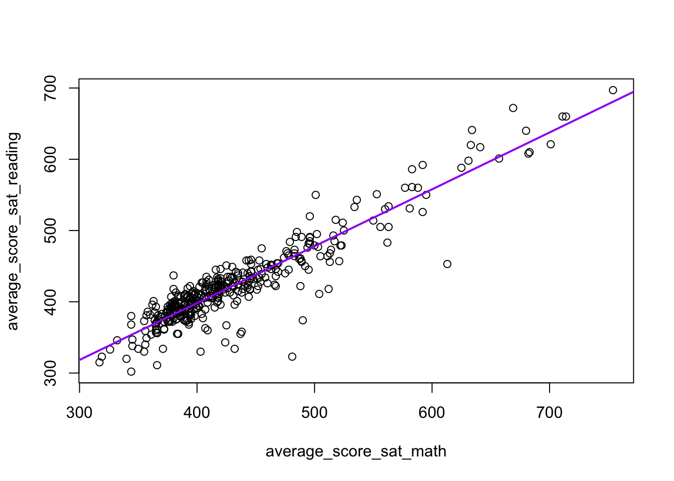
beta_0_hat <- ybar - xbar * beta_1_hatLet’s plot our data and our estimated regression line. We can plot the regression line using abline(). abline is similar to points/lines in that it needs to come after a call to plot. abline takes two required arguments a for the intercept and b for the slope.
plot(
  average_score_sat_reading ~ average_score_sat_math,
  data = nyc
)
abline(
  a = beta_0_hat, b = beta_1_hat,
  col = "purple", lwd = 2
)
6.1.1 Forecasting
We can use our fitted model to produce fitted values. For example, if we want to predict the average SAT reading score for a school with an average SAT math score of 450, we can do the following:
beta_0_hat + beta_1_hat * 450[1] 438.12Or, we can do in-sample prediction by using our dataframe
nyc$average_score_sat_reading_hat <- (beta_0_hat + beta_1_hat * nyc$average_score_sat_math)These, of course, will all fall on our line of best fit:
plot(
  average_score_sat_reading ~ average_score_sat_math,
  data = nyc
)
abline(
  a = beta_0_hat, b = beta_1_hat,
  col = "purple", lwd = 2
)
points(average_score_sat_reading_hat ~ average_score_sat_math, data = nyc, col = "purple")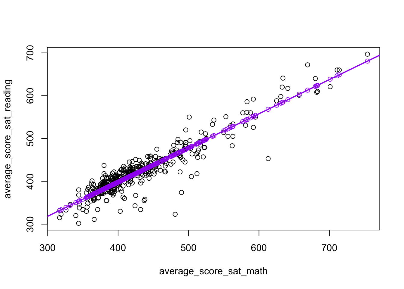
Another interesting property of regression is that \((\bar{X}, \bar{Y})\) will fall on the regression line. That is, the fitted value for a school with SAT math score of \(\bar{X}\) is \(\bar{Y}\):
ybar == beta_0_hat + beta_1_hat * xbar[1] TRUE6.1.1.1 Exercise
- Predict the SAT reading score for a school with an SAT math score of 600
6.2 First regression by function
Now, let’s compare our estimates to the ones produced by R’s built-in function lm. The lm function operates very similarly to plot: it takes two arguments: the formula y ~ x and the data argument. I will store the results of lm in a variable called est_lm so that I can use it in later functions.
## When lines get too long, use new lines to make reading the code easier
est_lm <- lm(
  average_score_sat_reading ~ average_score_sat_math,
  data = nyc
)
print(est_lm)
Call:
lm(formula = average_score_sat_reading ~ average_score_sat_math,
    data = nyc)

Coefficients:
           (Intercept)  average_score_sat_math
78.8797 0.7983 cat(paste0("\nbeta_0_hat = ", round(beta_0_hat, 4)))
beta_0_hat = 78.8797cat(paste0("\nbeta_1_hat = ", round(beta_1_hat, 4)))
beta_1_hat = 0.7983If we want more information, we pass est_lm to summary:
summary(est_lm)
Call:
lm(formula = average_score_sat_reading ~ average_score_sat_math,
    data = nyc)

Residuals:
     Min       1Q   Median       3Q      Max
-139.868   -9.486    2.426   13.195   71.166

Coefficients:
                       Estimate Std. Error t value Pr(>|t|)
(Intercept)            78.87972    7.26968   10.85   <2e-16 ***
average_score_sat_math  0.79831    0.01656   48.19   <2e-16 ***
---
Signif. codes:  0 '***' 0.001 '**' 0.01 '*' 0.05 '.' 0.1 ' ' 1

Residual standard error: 23.05 on 373 degrees of freedom
  (60 observations deleted due to missingness)
Multiple R-squared:  0.8616,    Adjusted R-squared:  0.8613
F-statistic:  2323 on 1 and 373 DF,  p-value: < 2.2e-16
As mentioned above, we will use the fixest package in this class. The function feols is equivalent to the lm function in base R and takes the same formula and data arguments. I will store the results of feols in a variable called est so that I can use it in later functions. To display the results, I will use the print function.
## Using fixest package
est <- feols(
  average_score_sat_reading ~ average_score_sat_math,
  data = nyc
)
NOTE: 60 observations removed because of NA values (LHS: 60, RHS: 60).print(est)OLS estimation, Dep. Var.: average_score_sat_reading
Observations: 375
Standard-errors: IID
Estimate Std. Error t value Pr(>|t|)
(Intercept) 78.879717 7.269680 10.8505 < 2.2e-16 ***
average_score_sat_math 0.798312 0.016565 48.1936 < 2.2e-16 ***
---
Signif. codes: 0 '***' 0.001 '**' 0.01 '*' 0.05 '.' 0.1 ' ' 1
RMSE: 23.0 Adj. R2: 0.8612576.2.1 Forecasting
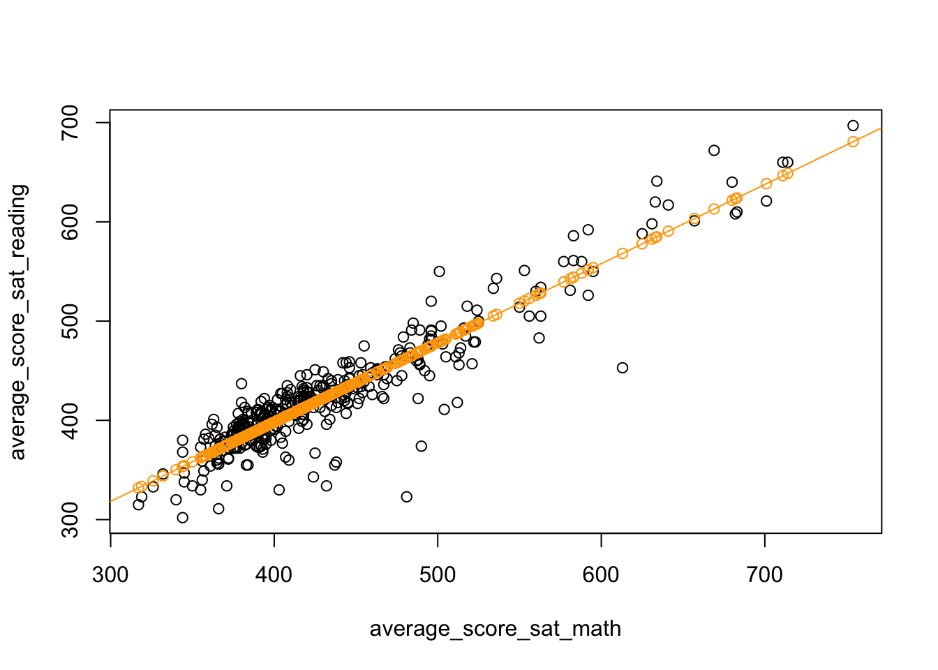
To forecast fitted values, we will use the predict function. The predict function takes as a first argument the result of lm or feols. In addition, we will use the newdata argument to use. The newdata argument must contain the same \(X\) variable(s) that we use in our regression.
# Predict yhat in-sample
nyc$yhat <- predict(est, newdata = nyc)

plot(
  average_score_sat_reading ~ average_score_sat_math, data = nyc
)
abline(coef = coef(est), col = "orange")
points(
  yhat ~ average_score_sat_math, data = nyc,
  col = "orange"
)
We can also forecast for different values by creating a new data.frame containing hypothetical values:
predict_df <- data.frame(average_score_sat_math = seq(300, 750, by = 10))
predict_df$yhat <- predict(est, newdata = predict_df)
plot(yhat ~ average_score_sat_math, data = predict_df)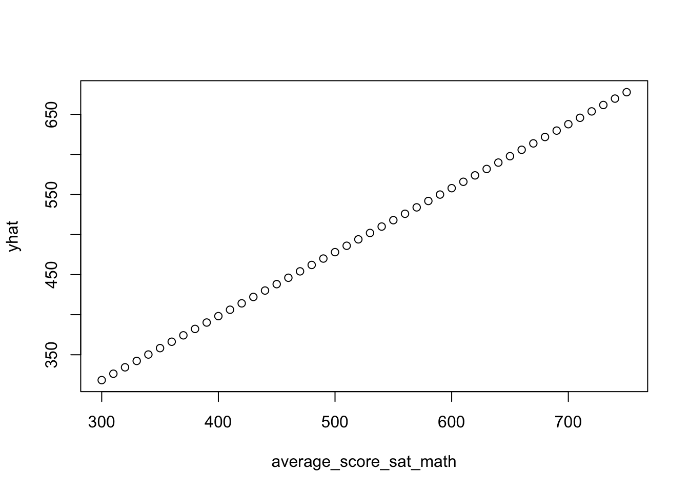
6.2.1.1 Exercise
- Run a regression of
average_score_sat_mathas the outcome variable andpercent_whiteas the predictor variable usingfeols. Interpret the coefficients in worlds
Answer:
- Create a plot of the raw data as well as the fitted regression line. Make sure each axis has high-quality labels.
6.2.2 Regression with indicator varaibles
feols(average_score_sat_math ~ 0 + i(borough), data = nyc)NOTE: 60 observations removed because of NA values (LHS: 60).OLS estimation, Dep. Var.: average_score_sat_math
Observations: 375
Standard-errors: IID
Estimate Std. Error t value Pr(>|t|)
borough::Bronx 404.357 6.82985 59.2044 < 2.2e-16 ***
borough::Brooklyn 416.404 6.47607 64.2989 < 2.2e-16 ***
borough::Manhattan 455.888 7.16687 63.6104 < 2.2e-16 ***
borough::Queens 462.362 8.13954 56.8045 < 2.2e-16 ***
borough::Staten Island 486.200 21.38083 22.7400 < 2.2e-16 ***
---
Signif. codes: 0 '***' 0.001 '**' 0.01 '*' 0.05 '.' 0.1 ' ' 1
RMSE: 67.2 Adj. R2: 0.114643feols(average_score_sat_math ~ i(borough), data = nyc)NOTE: 60 observations removed because of NA values (LHS: 60).OLS estimation, Dep. Var.: average_score_sat_math
Observations: 375
Standard-errors: IID
Estimate Std. Error t value Pr(>|t|)
(Intercept) 404.3571 6.82985 59.20435 < 2.2e-16 ***
borough::Brooklyn 12.0465 9.41203 1.27991 2.0138e-01
borough::Manhattan 51.5305 9.90005 5.20508 3.2223e-07 ***
borough::Queens 58.0052 10.62540 5.45911 8.7887e-08 ***
borough::Staten Island 81.8429 22.44519 3.64634 3.0411e-04 ***
---
Signif. codes: 0 '***' 0.001 '**' 0.01 '*' 0.05 '.' 0.1 ' ' 1
RMSE: 67.2 Adj. R2: 0.117004feols(average_score_sat_math ~ i(borough, ref = "Manhattan"), data = nyc)NOTE: 60 observations removed because of NA values (LHS: 60).OLS estimation, Dep. Var.: average_score_sat_math
Observations: 375
Standard-errors: IID
Estimate Std. Error t value Pr(>|t|)
(Intercept) 455.88764 7.16687 63.610428 < 2.2e-16 ***
borough::Bronx -51.53050 9.90005 -5.205076 3.2223e-07 ***
borough::Brooklyn -39.48397 9.65937 -4.087634 5.3483e-05 ***
borough::Queens 6.47468 10.84510 0.597014 5.5086e-01
borough::Staten Island 30.31236 22.55003 1.344227 1.7970e-01
---
Signif. codes: 0 '***' 0.001 '**' 0.01 '*' 0.05 '.' 0.1 ' ' 1
RMSE: 67.2 Adj. R2: 0.1170046.2.3 Interactions
workers <- read.csv("data/cps.csv")
str(workers)
'data.frame': 15992 obs. of 9 variables:
$ age : int 45 21 38 48 18 22 48 18 48 45 ...
$ education: int 11 14 12 6 8 11 10 11 9 12 ...
$ black : int 0 0 0 0 0 0 0 0 0 0 ...
$ hispanic : int 0 0 0 0 0 0 0 0 0 0 ...
$ married : int 1 0 1 1 1 1 1 0 1 1 ...
$ nodegree : int 1 0 0 1 1 1 1 1 1 0 ...
$ re74 : num 21517 3176 23039 24994 1669 ...
$ re75 : num 25244 5853 25131 25244 10728 ...
$ re78 : num 25565 13496 25565 25565 9861 ...workers$college <- 1 - workers$nodegreeFor interactions between two discrete variables, we need a special syntax:
feols(re78 ~ i(black, i.college), workers)OLS estimation, Dep. Var.: re78
Observations: 15,992
Standard-errors: IID
Estimate Std. Error t value Pr(>|t|)
(Intercept) 12817.225 146.402 87.548265 < 2.2e-16 ***
black::0:college::1 3153.177 173.126 18.213228 < 2.2e-16 ***
black::1:college::0 -2152.322 445.900 -4.826912 1.3995e-06 ***
black::1:college::1 216.947 396.580 0.547045 5.8436e-01
---
Signif. codes: 0 '***' 0.001 '**' 0.01 '*' 0.05 '.' 0.1 ' ' 1
RMSE: 9,510.4 Adj. R2: 0.02795For interactions between a discrete variable and a continuous variable,
feols(re78 ~ 0 + i(black) + i(black, age), workers)OLS estimation, Dep. Var.: re78
Observations: 15,992
Standard-errors: IID
Estimate Std. Error t value Pr(>|t|)
black::0 10610.336 247.64760 42.84449 < 2.2e-16 ***
black::1 7791.504 869.97852 8.95597 < 2.2e-16 ***
black::0:age 134.108 7.06422 18.98411 < 2.2e-16 ***
black::1:age 129.046 25.24742 5.11126 3.237e-07 ***
---
Signif. codes: 0 '***' 0.001 '**' 0.01 '*' 0.05 '.' 0.1 ' ' 1
RMSE: 9,499.7 Adj. R2: 0.0300796.2.3.1 Exercise
- Using a regression, what are the average earnings in 1975 (
re75) for Black workers, Hispanic workers, and White workers?
Answer:
- Use a regression to estimate the association of marriage and 1975 earnings. How much more do married people earn on average?
Answer:
- Use the results of this regression to determine whether the difference in earnings is larger for people with college degrees than those without.
feols(re75 ~ i(married, i.college), data = workers)OLS estimation, Dep. Var.: re75
Observations: 15,992
Standard-errors: IID
Estimate Std. Error t value Pr(>|t|)
(Intercept) 4527.51 209.946 21.5651 < 2.2e-16 ***
married::0:college::1 5152.80 259.519 19.8552 < 2.2e-16 ***
married::1:college::0 9951.44 257.785 38.6037 < 2.2e-16 ***
married::1:college::1 12024.03 229.335 52.4301 < 2.2e-16 ***
---
Signif. codes: 0 '***' 0.001 '**' 0.01 '*' 0.05 '.' 0.1 ' ' 1
RMSE: 8,378.4 Adj. R2: 0.18298Answer: